Solar’s margin for error just halved: what a ±5% tolerance band actually means

Every grid-connected generator of scale operates against a schedule: a block-by-block declaration, in 96 fifteen-minute blocks a day, of how much it will inject. Reality never matches the declaration exactly — clouds move, wind dies, inverters trip. The Deviation Settlement Mechanism (DSM) prices the difference, and the tolerance band is the allowance at its centre: deviations within the band are settled gently or not penalised; deviations beyond it attract charges that escalate with the size of the miss.

A tolerance band is therefore best understood as an error budget. It is the regulator’s answer to the question: how wrong is a forecast allowed to be before being wrong costs money? For India’s wind and solar fleet, the long-standing answer at the state level had been ±10% — generous enough that a competent day-ahead forecast, revised a few times intraday, kept most blocks inside the band. That answer is now changing, and Karnataka has moved first.

On June 24, 2026, the Karnataka Electricity Regulatory Commission notified new DSM regulations for the state. Three changes matter most:

• Solar’s band is halved: the tolerance band for solar generators drops from ±10% to ±5% of schedule. Wind retains ±10% — an explicit regulatory judgment that solar, with its more predictable resource, should be held to a tighter standard
• Sixteen schedule revisions a day: generators may revise their schedules up to 16 times daily, giving them a roughly 90-minute cadence to bring the declaration back in line with what the sky is actually doing
• Open-access forecasting obligations: the regulations rework forecasting and scheduling requirements for open-access participants — extending the discipline beyond utility-scale sellers to the consumers and traders who use the state network

None of these is a technicality. Together they redefine what operating a solar asset in Karnataka means: forecasting stops being a compliance formality performed once a day and becomes a continuous operating discipline with a direct cash consequence per block.

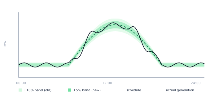
The intuitive reading — half the band, twice the exposure — understates the change, because forecast errors are not spread evenly. Solar forecast error distributions are peaked near zero with heavy tails: most blocks are nearly right, and a minority — cloud fronts, ramp hours, monsoon onset days — are badly wrong. Against a distribution shaped like that, the share of blocks falling outside ±5% is typically far more than double the share outside ±10%, because the band’s new edges cut into the fat body of the distribution, not just its tails. The penalty exposure scales non-linearly with the tightening.

The percentage arithmetic compounds the squeeze at the day’s edges. The band is defined relative to schedule — and during the morning and evening ramps, the schedule itself is small. A ±5% allowance on a plant scheduling 10% of capacity in an early block is a sliver of absolute megawatts, in exactly the hours when percentage errors are structurally largest: a fifteen-minute timing error in the sunrise ramp can be a 50% miss against a small denominator. Ramp-hour blocks were the main consumers of the old ±10% budget; under ±5%, they are where the penalties will concentrate.

The revision allowance is the counterweight to the tighter band — but only for operators equipped to use it. Sixteen revisions across the solar day means the schedule can be corrected roughly every hour and a half, and each revision typically takes effect a few blocks after submission. Used well, that converts intraday forecast skill directly into money: a plant that re-forecasts from live satellite imagery, sky cameras, and its own telemetry, and files a revision the moment the afternoon looks different from the morning’s view, resets its error to near zero many times a day. Used poorly — a day-ahead forecast filed at dawn and left to stand — the same plant carries a stale schedule into a ±5% band and pays for every hour of drift.

The gap between those two operators was modest under ±10%. Under ±5% it becomes the difference between a rounding error and a visible line in the plant’s revenue statement. The revision cadence is where the regulation quietly rewards operational sophistication.

Karnataka’s notification lands inside a national framework that is itself in motion. CERC’s move to link deviation settlement to the newly introduced reserve markets — pricing deviations against ancillary-service costs rather than exchange prices alone — was deferred to October 5, 2026, after grid operators flagged implementation concerns. And a suo-motu proceeding at CERC is re-determining the deviation “X” factor — the parameter that sets how much leeway wind and solar sellers get in the inter-state DSM formula — with effect from April 2026.

The deferral is a delay, not a retreat. Every element under review points the same direction: deviation charges more tightly coupled to the real cost of balancing the grid, and renewable-specific allowances narrowing as forecasting technology improves. The reasonable planning assumption for any RE seller is that today’s band is the loosest it will ever be.

DSM is layered: CERC’s regulations govern inter-state entities, while each State Electricity Regulatory Commission writes the rules inside its own borders. Karnataka moving to ±5% for solar does not move Tamil Nadu, Rajasthan, or Gujarat — each state updates on its own schedule, with its own bands, revision counts, and penalty formulas. For a developer or investor with assets across states, there is no longer a single number for “deviation risk.” The same megawatt of solar, with the same forecast quality, carries a different expected penalty in each state — and the ranking can flip each time a commission notifies new regulations.

This has two practical consequences. Portfolio valuation must price DSM exposure state by state, at the block level, under each state’s current rules — and stress it under plausible tightenings. And Karnataka’s move is best read as a template: state commissions watch one another, and a ±5% solar band that survives implementation in one large RE state tends to reappear in others’ draft regulations within a few cycles.

• Re-baseline forecast performance in dollars: the metric that matters is no longer MAE in percent but expected deviation charges per block under the new band. A forecast that was “good enough” at ±10% may be an open liability at ±5% — the only way to know is to replay historical generation against the new rules
• Invest in intraday, not just day-ahead: the 16-revision cadence means most of the recoverable value now sits in nowcasting — satellite, sky-camera, and telemetry-driven updates filed through the day. Day-ahead accuracy sets the starting point; revision discipline determines the bill
• Treat storage as a compliance instrument: a battery behind the meter can absorb the difference between actual and scheduled output in real time, keeping the plant inside the band during exactly the ramp blocks where forecasts fail — a revenue stream that did not exist at ±10% and that sizing studies should now price in
• Open-access consumers: your drawal schedule is now in scope: the reworked forecasting requirements pull open-access users into the same discipline. Consumption forecasting — shift patterns, process schedules, weather-driven load — becomes a scheduling input with a penalty attached, not an internal planning exercise
• Model the next amendment, not just this one: contracts and financial models built on today’s band will be marked to a tighter one. Sensitivity runs across band widths and penalty formulas separate assets that are robust to the regulatory trajectory from assets that merely comply with its current stop

The through-line from Karnataka’s notification to CERC’s proceedings is a single repricing: the grid is done absorbing renewable forecast error for free. Every percentage point of forecast accuracy, every well-timed schedule revision, and every block kept inside the band now has a dollar value that compounds across 35,040 blocks a year — and that value differs by state, by season, and by hour of day.

That is a block-level problem, and it demands block-level tools. EarthSync’s platform models deviation exposure at 15-minute resolution — replaying generation and consumption against each state’s actual DSM rules, current and drafted — so that generators, open-access consumers, and investors can see what a band change costs before the settlement statement delivers the answer. Karnataka has set the number at ±5%. The useful question is not whether the rest of the market follows, but whether your forecasts are ready when it does.